Spiking Neural Networks (SNNs) offer energy-efficient, biologically plausible computation but suffer from
non-differentiable spike generation, necessitating reliance on heuristic surrogate gradients. This paper
introduces UltraLIF, a principled framework that replaces surrogate gradients with
ultradiscretization, a mathematical formalism from tropical geometry providing continuous
relaxations of discrete dynamics. The central insight is that the max-plus semiring underlying
ultradiscretization naturally models neural threshold dynamics: the log-sum-exp function serves as a
differentiable soft-maximum that converges to hard thresholding as a learnable temperature parameter
ε → 0. Two neuron models are derived from distinct dynamical systems: UltraLIF
from the LIF ordinary differential equation (temporal dynamics) and UltraDLIF from the diffusion equation
modeling gap junction coupling across neuronal populations (spatial dynamics). Both yield fully
differentiable SNNs trainable via standard backpropagation with no forward-backward mismatch. Theoretical
analysis establishes pointwise convergence to tropical LIF dynamics with quantitative error bounds and
bounded non-vanishing gradients. Experiments on six benchmarks spanning static images, neuromorphic
vision, and audio demonstrate improvements over surrogate gradient baselines, with gains most pronounced
in the ultra-low latency regime (T=1) on neuromorphic and temporal datasets. An optional
sparsity penalty enables significant energy reduction while maintaining competitive accuracy.
Spike Mechanisms
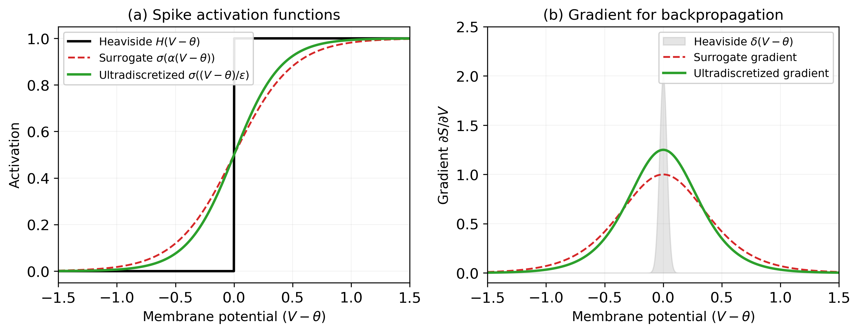
Figure 1. Spike activation functions and their gradients. (a) The Heaviside (hard threshold)
has zero gradient almost everywhere. Surrogate gradient methods replace it with a smooth proxy during
training only, creating a mismatch. UltraLIF uses the same smooth function in both forward and backward
passes — no mismatch by construction. (b) Gradients: UltraLIF provides bounded, non-vanishing
gradients for all membrane potentials.
Lay Summary
Spiking Neural Networks are brain-inspired AI models that communicate through brief electrical pulses,
making them far more energy-efficient than conventional AI. However, a fundamental training challenge has
persisted as an open problem: the “spike” is like an on/off switch, and on/off switches have
no smooth middle ground for standard learning algorithms to work with. Current methods work around this by
teaching the network using a smoothed approximation of the spike during training, then switching to the
real discrete spike at test time, creating a mismatch between how the model learns and how it actually
runs. This inconsistency is a known limitation of virtually all existing SNN training methods.
This work introduces UltraLIF, a spiking neuron derived from first principles using a mathematical
technique from physics called ultradiscretization. Rather than approximating the spike, the smooth
trainable operation emerges directly from the neuron’s governing equation, making training and
inference identical by construction. A temperature parameter, learned automatically during training,
controls how sharp each spike is and adapts to the complexity of the task.
UltraLIF outperforms existing methods across six benchmarks, including spoken word recognition,
moving-object detection from event-driven cameras, and standard image classification. It also scales
to larger, deeper architectures where conventional spiking neurons permanently switch off and stop
learning — a failure mode UltraLIF resolves through its self-adjusting firing sensitivity.
Interactive: Temperature Parameter ε
In UltraLIF, a single learnable parameter ε controls the softness of the spike function
s = σ(V / ε) and its gradient. Drag the slider to see
both effects simultaneously. At small ε the neuron fires sharply (near-binary), but
gradients become concentrated near the threshold. At large ε the response is smooth and
gradients are wide — but spikes lose discriminability.
Spike function — s = σ(V / ε)
ε = 1.00
Small ε → near-Heaviside. Large ε → gentle sigmoid.
Gradient — ∂s/∂V = s(1−s) / ε
same ε as left
Gradient is bounded for all ε > 0. No dead neurons.
The key advantage: unlike surrogate gradients (which are a different function from the forward
spike), UltraLIF’s gradient is the exact derivative of the same spike function used in the
forward pass — no mismatch.
Interactive: Membrane Update & Spike Scale
In standard UltraLIF a single ε does two jobs at once: it sets the softness of the
max-plus (LSE) membrane update and the spike sharpness (= 1/ε), so the
two are coupled. The decoupled variant (UltraLIF-DS) adds a separate spike scale β, giving
each parameter one clean role: ε = membrane smoothness and
β = spike sharpness, set independently. Drag ε to reshape the
membrane (left); drag β to sharpen the spike (right) without touching the membrane.
Membrane update — LSEε(a, 0) vs max(a, 0)
ε = 1.00
▮ LSE (soft max-plus)
⎯⎯ Hard max (ε→0)
Spike sharpness — s = σ(β · V)
β = 5.0
▮ σ(V/ε) standard
▮ σ(β · V) independent
⎯⎯ Heaviside
Gradient of LSE — ∂/∂a LSEε(a, 0) = σ(a/ε)
▮ LSE gradient
⎯⎯ Hard max gradient (step)
Spike gradients — ∂s/∂V for each curve
▮ (1/ε) σ(V/ε)(1−σ(V/ε))
▮ β σ(βV)(1−σ(βV))
In standard UltraLIF spike sharpness is locked to 1/ε, so you cannot sharpen the spikes
without also hardening the membrane. Decoupling adds β: ε keeps the membrane smooth
and trainable while β sharpens the spikes toward binary, independently.
Results: Ultra-Low Latency (T = 1)
The primary advantage of UltraLIF appears at a single timestep (T=1), where surrogate gradient
methods suffer most from forward-backward mismatch. Results below compare the best UltraLIF variant
against the best surrogate-gradient baseline on each dataset (1-layer FC, hidden=64, 100 epochs).
Gains are largest on temporally-structured data: +11.22% on spoken digits (SHD), +7.96% on event-camera
gestures (DVS-Gesture), +3.91% on spiking MNIST (N-MNIST).
Dataset
Type
Best Ultra (T=1)
Model
Best Baseline
Baseline Model
Gain
MNIST
Static
95.67%
UltraDLIF
95.58%
DSpike+
+0.09%
Fashion-MNIST
Static
83.02%
UltraPLIF
82.67%
DSpike+
+0.35%
CIFAR-10
Static
43.27%
UltraPLIF
40.26%
DSpike+
+3.01%
N-MNIST
Neuromorphic
94.14%
UltraDLIF
90.23%
DSpike
+3.91%
DVS-Gesture
Neuromorphic
60.23%
UltraPLIF
52.27%
PLIF
+7.96%
SHD
Audio spike
51.24%
UltraDLIF
40.02%
FullPLIF
+11.22%
Dataset
Best Ultra
Best Baseline
Gain (pp)
Relative gain
MNIST
95.67%
95.58%
+0.09
+0.1%
Fashion-MNIST
83.02%
82.67%
+0.35
+0.4%
CIFAR-10
43.27%
40.26%
+3.01
+7.5%
N-MNIST
94.14%
90.23%
+3.91
+4.3%
DVS-Gesture
60.23%
52.27%
+7.96
+15.2%
SHD
51.24%
40.02%
+11.22
+28.0%
Results: Depth Robustness (1L / 2L / 3L)
Standard LIF suffers dramatic accuracy collapse when depth increases at T=1, because forward-backward
mismatch compounds across layers. UltraLIF degrades minimally. The most striking example is SHD: adding
a second hidden layer causes LIF to collapse from 37.9% to 19.5% (−18.4pp), while UltraDLIF
drops only from 53.8% to 50.8% (−2.9pp). Ultra wins all 6 datasets at 3 layers, T=1.
2-Layer FC — T=1
Dataset
LIF
UltraDLIF
UltraDPLIF
UltraLIF
UltraPLIF
MNIST
95.97%
96.10%
96.10%
95.90%
96.22%
Fashion
82.65%
83.43%
83.43%
83.07%
83.45%
CIFAR-10
40.89%
44.20%
44.20%
43.44%
44.63%
N-MNIST
90.01%
94.94%
94.94%
90.74%
94.10%
DVS-Gesture
52.27%
51.52%
51.52%
53.41%
56.44%
SHD
19.48% (−18.4pp)
50.84%
50.84%
36.09%
42.01%
3-Layer FC — T=1
Dataset
LIF
UltraDLIF
UltraDPLIF
UltraLIF
UltraPLIF
MNIST
95.90%
96.22%
96.22%
95.63%
96.35%
Fashion
82.90%
83.55%
83.55%
82.23%
83.42%
CIFAR-10
40.35%
43.64%
43.64%
43.01%
44.15%
N-MNIST
87.82%
94.87%
94.87%
93.45%
93.68%
DVS-Gesture
50.38%
51.14%
51.14%
39.39%
43.94%
SHD
21.73%
45.67%
45.67%
24.25%
30.70%
Results: Energy Efficiency & Architecture Scalability
A sparsity penalty λ on the mean spike rate is added to the cross-entropy loss:
Loss = CE + λ · s̄. This directly reduces synaptic operations
(energy ∝ spike rate × T) with minimal accuracy cost, since UltraLIF’s learnable
ε can adapt to compensate.
Energy efficiency with sparsity penalty (λ = 0.1) — UltraPLIF across all datasets
Dataset
T
Acc. (λ=0)
Acc. (λ=0.1)
Spike rate (λ=0)
Spike rate (λ=0.1)
Reduction
MNIST
1
95.67%
95.71% ↑
0.445
0.268
40%
MNIST
10
97.35%
97.35%
0.473
0.239
50%
Fashion-MNIST
1
82.79%
83.05% ↑
0.428
0.266
38%
Fashion-MNIST
10
85.69%
85.74% ↑
0.456
0.279
39%
CIFAR-10
1
43.11%
43.04%
0.480
0.339
29%
CIFAR-10
10
45.75%
45.32%
0.469
0.340
28%
N-MNIST
10
97.38%
96.93%
0.475
0.292
39%
SHD
10
68.90%
70.27% ↑
0.469
0.383
18%
Architecture scalability across fully-connected (FC), convolutional (Conv), and ResNet backbones.
On ResNet50, standard LIF produces dead neurons at all timesteps while UltraLIF variants remain
stable, demonstrating that the self-adjusting ε resolves the dead neuron failure mode
even at large depth.
Architecture scalability — CIFAR-10
Architecture
T
LIF
Best Ultra
Model
Gain
FC 1-layer
1
41.79%
46.40%
UltraDPLIF
+4.61pp
FC 2-layer
1
40.89%
44.63%
UltraPLIF
+3.74pp
FC 3-layer
1
40.35%
44.15%
UltraPLIF
+3.80pp
Conv 2-layer
1
74.37%
70.54%
UltraDLIF
−3.83pp
ResNet18 + spiking FC
1
93.12%
93.37%
UltraLIF / UltraDPLIF
+0.25pp
ResNet18 + spiking FC
10
93.10%
93.50%
UltraLIF
+0.40pp
ResNet50 + spiking FC
1
31.83% (dead)
92.78%
UltraPLIF
+60.95pp
ResNet50 + spiking FC
5
35.09% (dead)
92.88%
UltraPLIF
+57.79pp
ResNet18 backbone — all datasets (T=1 / T=5 / T=10)
Dataset
LIF T=1
Best Ultra T=1
LIF T=5
Best Ultra T=5
LIF T=10
Best Ultra T=10
CIFAR-10
93.12%
93.37% (UltraLIF)
93.01%
93.39% (UltraDLIF)
93.10%
93.50% (UltraLIF)
Fashion-MNIST
93.81%
93.95% (UltraPLIF)
93.65%
93.89% (UltraDPLIF)
93.86%
94.24% (UltraDLIF)
N-MNIST
99.20%
99.23% (UltraDLIF)
99.13%
99.23% (UltraDLIF)
99.13%
99.23% (UltraDLIF)
ResNet50 backbone — CIFAR-10 (T=1 / T=5 / T=10)
Model
T=1
T=5
T=10
LIF
31.83% (dead)
35.09% (dead)
23.23% (dead)
UltraDLIF
92.23%
92.41%
92.54%
UltraDPLIF
92.22%
92.73%
90.42%
UltraLIF
91.92%
91.85%
91.77%
UltraPLIF
92.78%
92.88%
92.82%
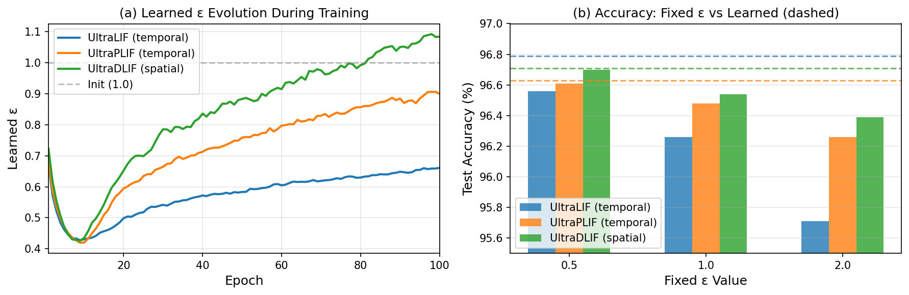
Figure. Epsilon ablation on MNIST (T=1, 100 epochs). Learned ε shows a
characteristic trajectory: initial sharpening then recovery to a model-specific optimum. Learned
ε consistently matches or exceeds all fixed configurations across all four UltraLIF variants.
Citation
@inproceedings{minoza2026ultralif,
  title     = {UltraLIF: Fully Differentiable Spiking Neural Networks
               via Ultradiscretization and Max-Plus Algebra},
  author    = {Mi{\~n}oza, Jose Marie Antonio},
  booktitle = {International Conference on Machine Learning},
  year      = {2026},
}