The SPIKE Architecture
SPIKE architecture: a PINN encoder maps (x, y, t) to the solution u, lifted into an observable space by a polynomial library plus a learned latent embedding, where a continuous-time Koopman operator enforces sparse linear dynamics.

Figure 1. A standard PINN encoder maps coordinates (x, y, t) to the solution field u. A dual observable embedding — an explicit polynomial library ψpoly plus a learned latent map ψlatent — lifts u into a space where a continuous-time Koopman operator enforces linear dynamics dz/dt = Az. An L1 penalty on A drives it toward a sparse, interpretable generator (heatmap, right).

Abstract

Physics-Informed Neural Networks (PINNs) solve differential equations mesh-free by embedding physical constraints into training, but they tend to overfit the training domain and generalize poorly when extrapolating beyond it. SPIKE (Sparse Physics-Informed Koopman-Enhanced) regularizes PINNs with continuous-time Koopman operators to learn parsimonious dynamics. By enforcing linear dynamics dz/dt = Az in a learned observable space, both PIKE (without explicit sparsity) and SPIKE (with L1 regularization on A) learn sparse generator matrices, embodying the parsimony principle that complex dynamics admit low-dimensional structure. Across parabolic, hyperbolic, dispersive, and stiff PDEs, including fluid dynamics (Navier–Stokes) and chaotic ODEs (Lorenz), SPIKE delivers consistent gains in temporal extrapolation, spatial generalization, and long-term prediction accuracy. The continuous-time formulation with matrix-exponential integration provides unconditional stability for stiff systems.

184×
longer valid prediction horizon on the chaotic Lorenz attractor (12.1 s vs 0.07 s)
5.5×
lower out-of-distribution MSE on Navier–Stokes downstream channel flow
5.7×
fewer non-zero generator entries under L1 sparsity (Schrödinger)
Key Ideas
koopman as regularizer

PINN-first, not Koopman-first

Rather than bolting physics onto a Koopman autoencoder, SPIKE keeps the PINN as the base model and adds Koopman structure as an auxiliary regularizer that promotes sparse, interpretable dynamics.

parsimony principle

Sparse generators

L1 regularization on A reduces non-zero entries by up to 5.7×, capturing complex PDE dynamics with sparse generator matrices — and even fixing unstable spectra (reaction-diffusion).

library + latent

Dual observable embedding

An explicit polynomial library (capturing terms like u−u³) combines with a learned latent map that correlates with hidden structure — up to 0.99 with uxx.

continuous time

Generator, not propagator

Learning dz/dt = Az directly avoids the diagonal-dominance trap of discrete-time Koopman (K → I as Δt → 0). Matrix-exponential integration gives unconditional stability.

Generalization Beyond the Training Domain

Solutions stay accurate not only in-domain but when extrapolating in time. The shaded panels (red) sit outside the training window t∈[0,1].

Solution comparison for Burgers and advection equations at t = 0.3, 0.6, 0.9 (in-domain) and t = 1.5 (out of distribution). All Koopman-regularized variants track the analytical solution into the OOD region.

Figure 2. In-domain vs. out-of-distribution solutions. Burgers (top) and advection (bottom) at increasing times. Every method matches the analytical solution in-domain; the regularized variants continue to track it at t=1.5, beyond the training window.

Chaos & Fluids
Animated Lorenz attractor. The baseline PINN diverges from the chaotic trajectory almost immediately, while SPIKE-EXPM stays valid far longer.

Lorenz attractor. The continuous-time Koopman variant (SPIKE-EXPM) stays within the error threshold for 12.1 s versus 0.07 s for the baseline PINN — an order-of-magnitude longer horizon on a chaotic system.

Animated Navier-Stokes channel flow comparison over time. PIKE-EXPM achieves 5.5x lower downstream out-of-distribution MSE than the PINN baseline.

Navier–Stokes channel flow. Predicting downstream (x∈[1,2]) of the training region, PIKE-EXPM reaches 7.1×10⁻² MSE vs. the PINN's 3.9×10⁻¹ — a 5.5× reduction.

Quantitative Results

Physics-residual MSE (lower is better) across systems and generalization regimes, plus Koopman diagnostics. Best per row in blue. Full results for all systems are in the repository.

Summary of Key Improvements over the PINN Baseline (grouped by metric type)

SystemMetricImprovementBest Method
In-Domain MSE
2D Wavein-domain8×107×PIKE-Euler
Cahn-Hilliardin-domain106×PIKE-Euler
OOD-Space MSE (extrapolation beyond training domain)
2D Burgersxy ∈ [1,2]38×PIKE-Euler
Advectionx ∈ [3,5]29×SPIKE-EXPM
Allen-Cahnx ∈ [3,5]7.5×PIKE-Euler
Navier-Stokesxy ∈ [1,2]32×PIKE-Euler
Kuramoto-Sivashinskyx ∈ [3,5]2.1×SPIKE-EXPM
OOD-Time MSE
Schrodingert ∈ [3,5]24×SPIKE-EXPM
KdVt ∈ [3,5]6.3×PIKE-EXPM
Burgerst ∈ [3,5]2.4×PIKE-Euler
Kuramoto-Sivashinskyt ∈ [3,5]2.8×PIKE-RK4
Chaotic Systems (Valid Prediction Time)
Lorenzvalid time184×PIKE-Euler

Bounded-domain problems where spatial extrapolation demonstrates model capability rather than physical prediction. Improvement = PINN MSE / best-method MSE (higher is better).

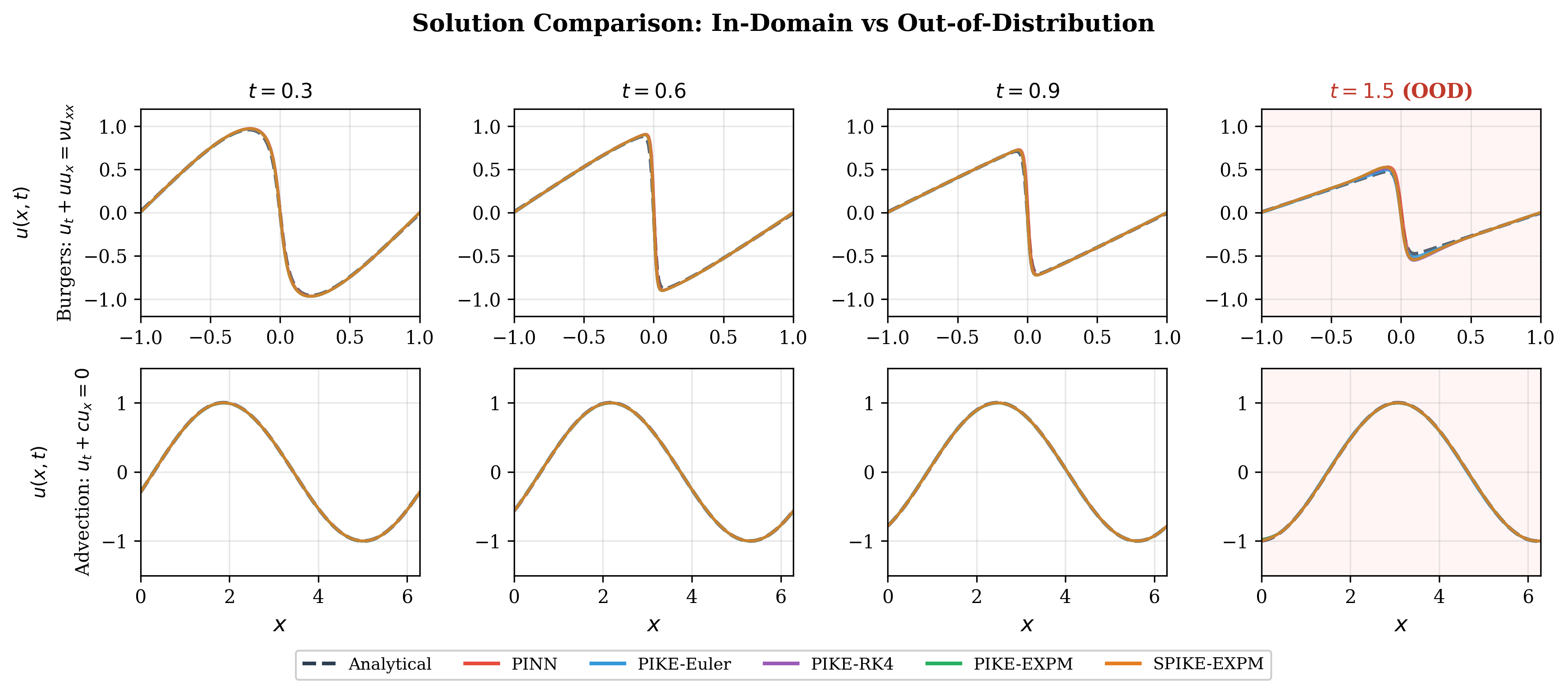
1D PDEs — In-Domain Physics Residual MSE (x, t ∈ [0,1])

PDEPINNPIKE-EulerPIKE-RK4PIKE-EXPMSPIKE-EXPM
heat1.01e-56.95e-61.20e-56.02e-68.67e-6
advection5.04e-78.89e-54.45e-74.88e-73.90e-7
burgers9.68e-54.63e-53.44e-53.23e-53.23e-5
allen-cahn1.19e-51.56e-51.44e-52.34e-57.08e-5
kdv5.23e-24.75e-25.24e-25.06e-25.14e-2
reaction-diffusion5.02e-52.67e-44.80e-54.63e-51.51e-4
cahn-hilliard3.53e-12.61e-73.50e-13.46e-11.22e-1
kuramoto-sivashinsky1.83e+18.77e+16.75e+22.93e+21.91e+1
schrodinger2.50e+12.53e+12.49e+12.47e+11.20e+1

1D PDEs — Spatial Extrapolation (OOD-Space) (x ∈ [1,3], t ∈ [0,1])

PDEPINNPIKE-EulerPIKE-RK4PIKE-EXPMSPIKE-EXPM
heat1.64e-31.09e-31.71e-31.69e-31.66e-3
advection4.50e-71.86e-52.87e-73.13e-71.98e-7
burgers5.90e-31.80e-26.59e-36.10e-36.10e-3
allen-cahn4.50e-25.89e-25.02e-25.85e-26.17e-2
kdv2.63e-22.57e-22.64e-22.64e-22.63e-2
reaction-diffusion5.55e-52.71e-35.82e-57.29e-53.97e-5

1D PDEs — Temporal Extrapolation (OOD-Time) (x ∈ [0,1])

PDEPINNPIKE-EulerPIKE-RK4PIKE-EXPMSPIKE-EXPM
t ∈ [1, 3]
heat1.82e-41.64e-41.94e-41.80e-41.79e-4
advection3.10e-71.23e-53.72e-73.20e-73.89e-7
burgers8.10e-23.09e-21.12e-18.93e-28.93e-2
allen-cahn2.04e-22.33e-21.93e-22.37e-22.35e-2
kdv2.28e-23.48e-22.17e-21.78e-21.89e-2
reaction-diffusion2.00e-34.20e-32.10e-32.27e-32.31e-3
t ∈ [3, 5]
heat7.52e-42.17e-37.00e-47.97e-48.03e-4
advection4.05e-102.96e-96.02e-104.48e-101.06e-9
burgers2.77e-21.15e-22.97e-22.91e-22.91e-2
allen-cahn6.21e-21.11e-16.46e-29.76e-29.58e-2
kdv8.89e-32.49e-29.99e-31.42e-31.81e-3
reaction-diffusion9.72e-31.73e-21.06e-21.17e-21.12e-2

2D PDEs — In-Domain Physics Residual MSE (x, y, t ∈ [0,1])

PDEPINNPIKE-EulerPIKE-RK4PIKE-EXPMSPIKE-EXPM
wave 2D1.72e+42.06e-42.17e+57.69e+45.11e-2
burgers 2D9.66e-37.12e-34.92e-23.23e-29.34e-3
navier-stokes 2D1.81e-11.43e-12.58e-13.59e-11.56e-1

Navier–Stokes — Downstream Channel Flow (physically meaningful OOD, t = 0.5)

RegionPINNPIKE-EulerPIKE-RK4PIKE-EXPMSPIKE-EXPM
in-domain (x ∈ [0,1])2.06e-13.74e-11.55e-14.64e-29.06e-2
OOD-downstream (x ∈ [1,2])3.94e-15.06e-13.32e-17.14e-21.62e-1

PIKE-EXPM achieves a 5.5× lower OOD-downstream MSE than PINN (7.14e-2 vs 3.94e-1).

Chaotic Dynamics — Lorenz Lyapunov Analysis λ = 1.1 s)

MetricPINNPIKE-EulerPIKE-RK4PIKE-EXPMSPIKE-EXPM
Valid time (s) ↑0.0712.120.0712.1212.12
τ ratio ↑0.0611.020.0611.0211.02
Short-term MSE ↓2.31e+11.60e-11.93e+16.16e-16.16e-1

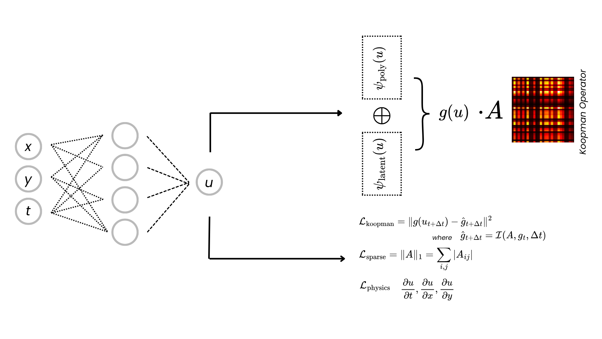
Koopman Latent R² (higher is better; PIKE/SPIKE only)

SystemPIKE-EulerPIKE-RK4PIKE-EXPMSPIKE-EXPM
heat0.99890.99890.99900.9990
advection0.88950.90040.90030.9003
burgers0.96990.96700.96950.9695
allen-cahn0.99830.99830.99830.9982
kdv0.92470.94810.94950.9471
reaction-diffusion0.98270.98950.98950.9857
burgers 2D0.95800.95030.97560.9550
navier-stokes 2D0.80080.90410.89310.8750

Learned Dynamics Structure (interpretability: library term + latent correlations)

PDETrue equationLibrary dg1/dtLatent correlations
Heatut = α uxx+0.07 g2uxx (0.99)
Advectionut = −c ux0ux (0.96), ut (0.96)
Burgersut = −u ux + ν uxx−0.06 g0 + 0.04 g1u−u³ (0.97), uxx (0.27)
Allen-Cahnut = ε uxx + u − u³+0.03 g0 − 0.03 g1u−u³ (0.85), uxx (0.57)
KdVut = −u ux − uxxx0u³ (1.00), uxx (0.94)
Reaction-Diffusionut = D uxx + R(u)−0.03 g0 + 0.01 g1uxx (0.76), u³ (0.91)
Kuramoto-Sivashinskyut = −u ux − uxx − uxxxx≈ 0 (4× sparser)u³ (0.96), uxx (0.38)
Schrodingeri ut = uxx + |u|² u−0.01 g0ure (0.55), |u|² (0.36)

Observable convention g0 = 1, g1 = u, g2 = u². Bold marks strong latent correlations (|r| > 0.7). The sparse generator recovers interpretable structure: SPIKE's L1 penalty makes Kuramoto-Sivashinsky 4× sparser while preserving the dominant u³ coupling.

Method Variants

Choosing an Integrator (stability–accuracy tradeoff vs. PDE stiffness)

IntegratorStabilityAccuracyOverheadRecommended when
EulerConditionalO(Δt)MinimalNon-stiff PDEs (heat, advection, Burgers)
RK4Conditional (larger region)O(Δt4)~5%Moderate stiffness requiring higher accuracy
EXPMUnconditionalExact for linear~25%Stiff PDEs (Cahn-Hilliard, KS, Schrodinger)

Practical guideline: start with PIKE-Euler; if instability appears (oscillations, divergence) or the PDE has fourth-order spatial derivatives, switch to EXPM. For non-stiff systems Euler often achieves the tightest Koopman fit; for stiff systems (max| > 104) EXPM's unconditional stability justifies its ~25% overhead.

Citation
@InProceedings{pmlr-v328-minoza26a,
  title     = {SPIKE: Sparse Koopman Regularization for Physics-Informed Neural Networks},
  author    = {Mi\~{n}oza, Jose Marie Antonio},
  booktitle = {Conference on Parsimony and Learning},
  pages     = {164--191},
  year      = {2026},
  editor    = {Burkholz, Rebekka and Liu, Shiwei and Ravishankar, Saiprasad
               and Redman, William and Huang, Wei and Su, Weijie and Zhu, Zhihui},
  volume    = {328},
  series    = {Proceedings of Machine Learning Research},
  month     = {23--26 Mar},
  publisher = {PMLR}
}